

Field Verifications – Getting More Bang for Your Buck


Discussing ways of refining field measurements to help improve integrity management.
Metal loss corrosion reduces the lifespan of our assets. As the industry seeks to extend asset life, it is fundamental that we manage integrity to ensure we assess the significance of metal loss corrosion. The challenge is to identify if any feature threatens safe operation. To do this, we need to estimate when a feature may grow to critical dimensions. Assessment of the significance of metal loss corrosion is reliant on accurate estimates of feature dimensions.
The results of these assessments are used to help operators make effective decisions in managing the integrity of their assets. For this reason, uncertainties in the estimates of feature dimensions can affect the accuracy of decision-making.
So, how do we achieve all this? The techniques described in this article can be used to refine estimates of feature dimensions, and help make efficient integrity management decisions for our assets.
Measurements and Tolerances
For pipelines, the dimensions of metal loss corrosion features may be indirectly measured using inline inspection (ILI) methods, such as magnetic flux leakage or ultrasonic technologies. Sizing of the dimensions of these features is associated with measurement tolerance and a degree of uncertainty.
It is common practice to allow for tolerances and safety factors when engineers assess whether flaws are acceptable to given criteria (for example, a maximum allowable operating pressure). Clearly, this is conservative because, by including tolerances, we assess the worst-case scenario for our corrosion features.
When identifying features that pose a threat to integrity, we need to make a decision on how best to manage them. Sometimes, we have no alternative but to physically examine our assets and use direct measurement techniques to examine the critical features in more detail. In many cases, features need to be dug up for repair. Having these features measured for their accurate dimensions is a common practice. There are a number of ways to measure the dimensions of critical features in the field. Some of the methods used, such as ultrasonics, can provide very accurate measurements with low tolerances. These measurements can be used to help re-assess criticality and decide if any final actions are needed, such as a repair. The trade-off for high accuracy is that field measurements need to be scheduled, they require skilled personnel, are time-consuming and can cost a lot of money. Normally, the final decision on what to do with the measured feature dimensions following field measurements is the end of the story. But, it does not have to be. One can use the results of the field measurements to examine its ILI or ILI results. In some situations, field measurements can be used to help re-assess features reported by ILI. This can be very useful for a number of reasons, such as scheduling field digs and measurements, scheduling ILI campaigns, and can help gain more insight into the criticality of the most significant features.
Bias
When comparing the field measurement results with the ILI results, one can find a difference between them. When this is consistent, we can say that there is a bias. There are many reasons for a difference between the ILI and field measurements; for instance, certain types of features may be harder for ILI tools to size compared to others. Variations can also be due to inspection tool technologies and their associated sizing accuracies and differences between ILI and field measurement tools.
Where we think there may be a bias, we can use some maths to see if it is significant or not. This involves comparing two sets of measurements and checking the degree of difference between them. This is something that is commonly carried out in other industries, such as clinical research trials. In fact, the methods used – in the oil and gas industry – to investigate bias are based on medical assessments, to check for agreement between two or more sets of measurements.
Clearly, we need enough field and ILI data measurements to enable to check for bias. It is also important to understand that bias can work in two ways. For example, ILI results can either over or under-call feature lengths, compared to field measurements.
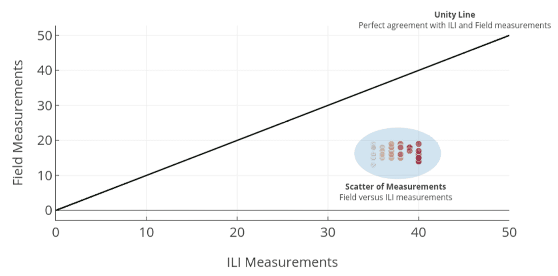
The first step in checking for bias is to plot field measurements against the corresponding ILI measurements. An example of this is shown in Figure 1. These measurements could relate to any dimension, for instance, depths, lengths or widths.
The values can be used to identify trends and measure how different the field and ILI measurements are from each other (Figure 1). If the field and ILI measurements were exactly the same, they would all lie on the line of unity. However, in this case, we can see a clear trend: the ILI has consistently over-called in comparison to the field measurements.
In order to estimate how different the results may be, we need to compare the difference between each field and ILI measurement against the average.
Measurements of Bias
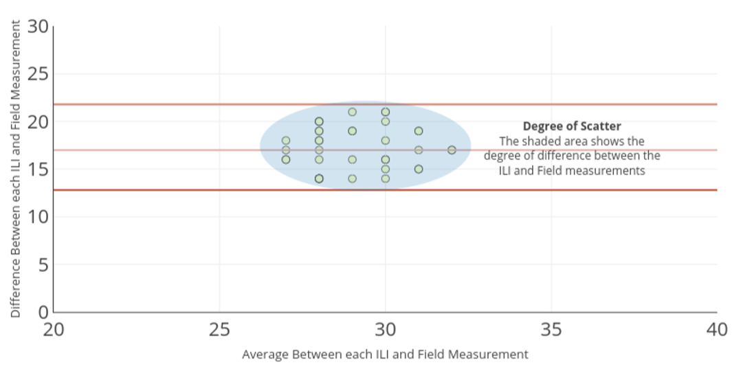
The data can be examined in more detail by plotting the difference between each ILI and field measurement against their average value or mean.
To give us a sense of how different the measurements are, we can plot the mean of differences and set some acceptable upper and lower bounds. In Figure 2, the mean of differences between ILI and field measurements is plotted as along the centre of the graph. The acceptable upper and lower bounds are plotted near the top and bottom. In this case, the acceptable bounds are the commonly used ‘two standard deviations from the mean’ test statistic.
The extent of scatter (represented by the shaded area in Figure 2) shows what the degree of difference is between the ILI and field measurements. So, in this example, we can check what the degree of difference could reasonably be by looking at the upper and lower bounds on the y-axis, i.e. anywhere roughly between 12.5 and 22. This result shows that there is bias between the ILI and field measurements and what values the difference lies between.
On the other hand, if we find the scatter is centred on the x-axis, it shows that there is no bias between the measurements. Plots like this provide an easy way to examine data and to check what bias if any exists. They also let us check what the extent of the difference may be.
It is commonly found that the differences between ILI and field measurements are normally distributed. Provided there are enough field measurements, one can analyse if there is any significant degree of difference and, if so, how big that difference is. One can also work out how accurate the difference is by calculating a standard error.
Degree of Difference
There are a number of ways to work out how different the ILI and field measurements may be. One common way of calculating differences is to look at measurement variances. This is a formalised statistical method called analysis of variance (ANOVA).
ANOVA techniques use well-established tests to work out if the average of one set of measurements is significantly different from the average of another. One of the advantages of using ANOVA in this way is that it gives a measure of confidence in any difference.
An example would be, if one’s ANOVA tests illustrate we are very confident (e.g. 99%) that the ILI measurements have over-called the field measurements, then we can re-assess feature criticality. In turn, one is able to make more effective decisions to manage integrity.
Generally, one’s confidence to accept or reject the bias increases with the number of field measurements. Although there is no hard and fast rule for the number of digs needed to be carried out to give confidence in any bias, past a certain amount, the value from any one dig becomes progressively lower. However, a clear bias can generally be seen within a few field measurements. This process, in turn, helps to minimise the number of excavations required in the future and, in some cases, can eliminate the need to carry out some digs altogether. In addition, it may help to gain a greater understanding into what corrosion mechanisms may exist. Having an optimal number of excavations is key to this methodology.
Considerations
Bias and ANOVA techniques provide another set of tools to help make informed decisions about managing the integrity of one’s assets. Used in the right way, they let us use the results of field measurements in feedback with ILI measurements, to provide a greater understanding of critical features that may threaten safe operation. The results of the bias and ANOVA methods can be updated in real time as field measurements become available, and can use these to efficiently schedule dig campaigns. This methodology helps to remove some unnecessary conservatism associated with the assessments. It also makes use of field measured values, which otherwise would be unused, to help refine one’s integrity assessments and to efficiently prioritise future digs.
Table 1 - Example data set with ILI measured depth and corresponding field measured value
Exam
An example where a set of ILI measurements is compared with corresponding field measurements is shown in Table 1.
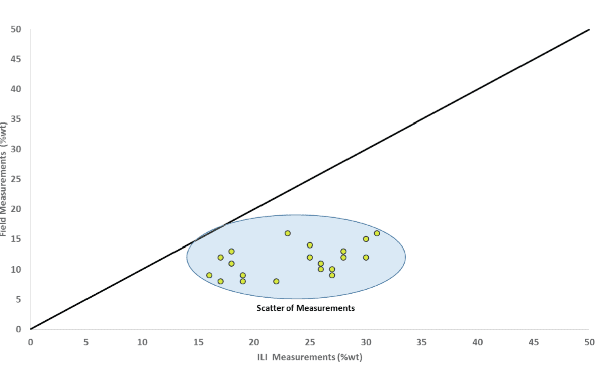
Figure 3 shows the above ILI measurements against their corresponding field measurements. The scatter of measurements is marked by the blue shaded area. In this case, the ILI measurements have over-called the depth values compared to the field measurements, as all the points lie below the line of unity.
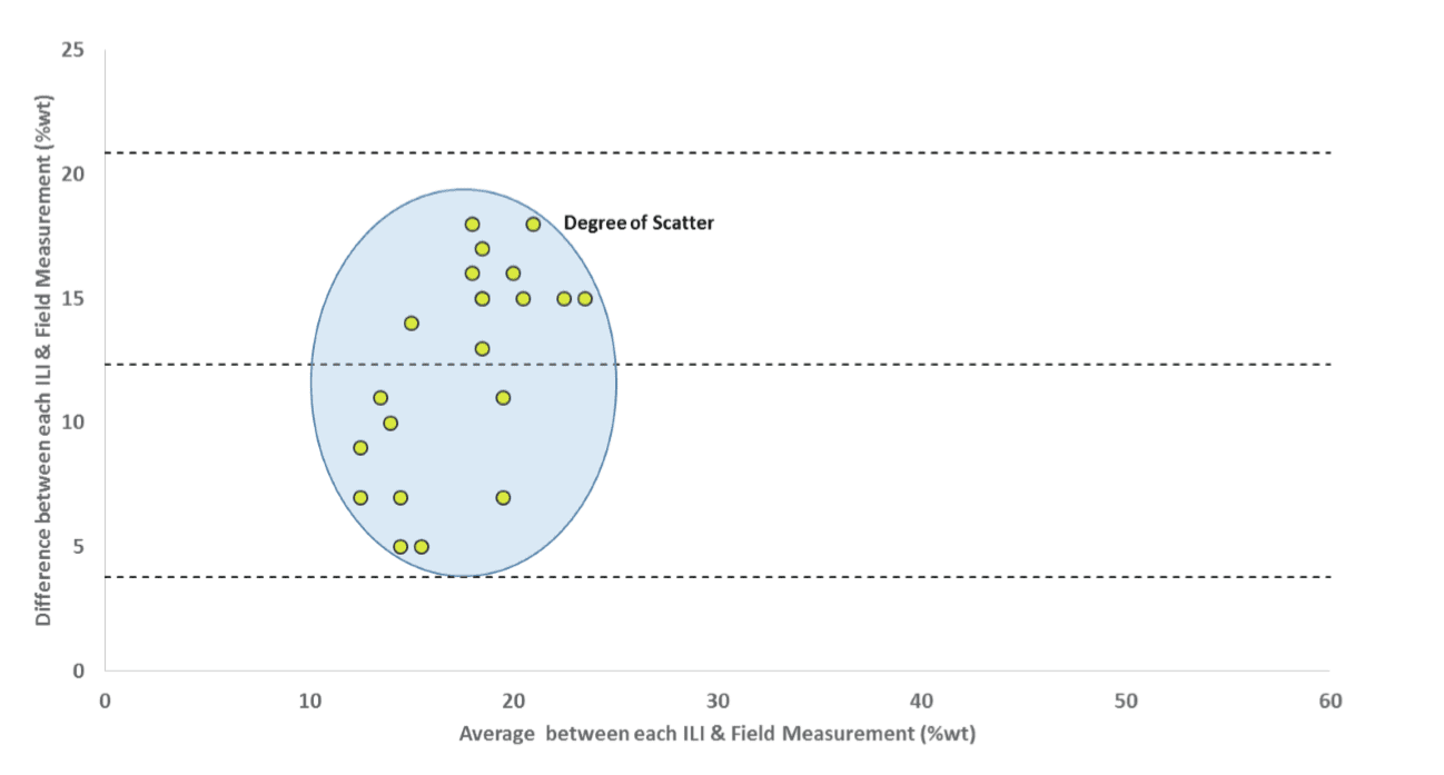
Figure 4 shows the plot of difference between each ILI and field measurement against their average value; a clear bias in the data with an average (of differences) of 12.3% of wall thickness is shown by the central, horizontal line.
In this case, ANOVA calculations show that we have a 99.9% confidence that the means between the ILI and field measurements are different. Although data used in this example is fictitious, it is based on a real life example.
Insights & News

Exceedance Probability Modeling in Pipeline Integrity Using Big Data Techniques for Crack Type Anomalies
In our latest technical insight, Penspen Asset Integrity experts explore how exceedance probability modelling and big data techniques can be applied to crack-type anomalies to support risk-based...

Mitigating Intermittency: Practical Strategies for Green Ammonia Production in Off-Grid Environments
In our latest insight, Penspen’s Nigel Curson explores practical strategies for designing off-grid green ammonia facilities, from renewable hybridisation and energy storage to system optimisation...
A Pragmatic Framework for Prioritising Hydrogen Repurposing Actions in Complex Pipeline Systems
Presented for the first time at the 2026 Pipeline Technology Conference, our latest technical insight introduces a practical, risk-informed framework for prioritising hydrogen repurposing actions...

From Academia to Industry: Ronald’s Journey into Pipeline Integrity Excellence
Based in Bogota, Colombia, a life-long fascination with mathematics has driven Ronald to pursue a career where data is crucial for the safe operations of energy...
Penspen Launches Three New Asset Integrity Training Courses in the Middle East & Africa Region
Penspen has launched three new Asset Integrity online training courses across the Middle East & Africa (MEA) region, supporting operators in strengthening pipeline integrity and managing ageing...

Penspen Awarded Hydrogen Transition Pathways for Industrial Clusters Study
International energy consultancy Penspen has been awarded a critical research project designed to look into how hydrogen can support the transition of the UK’s industrial clusters. Hydrogen...

Penspen Shortlisted for Large Company of the Year at 2026 Gas Industry Awards
Penspen has been shortlisted as a finalist for the Large Company of the Year award at the 2026 Gas Industry Awards. The awards, organised by the Institution of Gas Engineers & Managers (IGEM) and...
More insights
-
Exceedance Probability Modeling in Pipeline Integrity Using Big Data Techniques for Crack Type Anomalies
In our latest technical insight, Penspen Asset Integrity experts explore how exceedance probability modelling and big data techniques can be applied to crack-type anomalies to support risk-based pipeline…
Read insight -

Mitigating Intermittency: Practical Strategies for Green Ammonia Production in Off-Grid Environments
In our latest insight, Penspen’s Nigel Curson explores practical strategies for designing off-grid green ammonia facilities, from renewable hybridisation and energy storage to system optimisation approaches that improve…
Read insight